Solution Manual for Forecasting and Predictive Analytics with Forecast X, 7th Edition

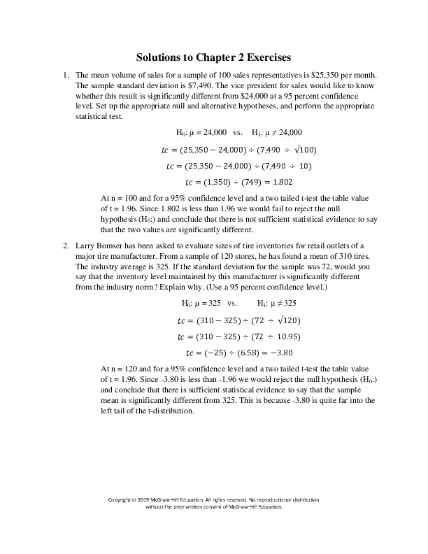
Solutions to Chapter 2 Exercises 1. The mean volume of sales for a sample of 100 sales representatives is $25,350 per month. The sample standard deviation is $7,490. The vice president for sales would like to know whether this result is significantly different from $24,000 at a 95 percent confidence level. Set up the appropriate null and alternative hypotheses, and perform the appropriate statistical test. H0: µ = 24,000 vs. H1: µ ≠ 24,000 ?? = (25,350 − 24,000) ÷ (7,490 ÷ √100) ?? = 25,350 − 24,000 ÷ 7,490 ÷ 10 ?? = 1,350 ÷ 749 = 1.802 At n = 100 and for a 95% confidence level and a two tailed t-test the table value of t = 1.96. Since 1.802 is less than 1.96 we would fail to reject the null hypothesis (H0:) and conclude that there is not sufficient statistical evidence to say that the two values are significantly different. 2. Larry Bomser has been asked to evaluate sizes of tire inventories for retail outlets of a major tire manufacturer. From a sample of 120 stores, he has found a mean of 310 tires. The industry average is 325. If the standard deviation for the sample was 72, would you say that the inventory level maintained by this manufacturer is significantly different from the industry norm? Explain why. (Use a 95 percent confidence level.) H0: µ = 325 vs. H1: µ ≠ 325 ?? = (310 − 325) ÷ (72 ÷ √120) ?? = 310 − 325 ÷ 72 ÷ 10.95 ?? = −25 ÷ 6.58 = −3.80 At n = 120 and for a 95% confidence level and a two tailed t-test the table value of t = 1.96. Since -3.80 is less than -1.96 we would reject the null hypothesis (H0:) and conclude that there is sufficient statistical evidence to say that the sample mean is significantly different from 325. This is because -3.80 is quite far into the left tail of the t-distribution. Copyright © 2019 McGraw-Hill Education. All rights reserved. No reproductionor distribution without the prior written consent of McGraw-Hill Education. 3. Twenty graduate students in business were asked how many credit hours they were taking in the current quarter. Their responses are shown as follows (c2p3): Student Number 1 2 3 4 5 6 7 8 9 10 Credit Hours 2 7 9 9 8 11 6 8 12 11 Student Number 11 12 13 14 15 16 17 18 19 20 Credit Hours 6 5 9 13 10 6 9 6 9 10 1. Determine the mean, median, and mode for this sample of data. Write a sentence explaining what each means. Mean = 8.3 Median = 9 Mode = 9 The mean is the arithmetic average which is equal to the sum of the observations (166) divided by the number of observations (20). That is, (166/20) = 8.3. The median is the middle value that splits the data into two equal parts when the data are arrayed from low to high (or high to low). In this case sorting from low to high would show us that observations 10 through 14 are all equal to 9. When there are an even number of observations there is no middle value. In such a case one uses the average of the two most middle values, which in this case are both 9 (observations 10 and 11). Thus, the median is 9. The mode is the most frequently occurring value. In this sample there are five observations equal to 9. The next most would be a value of 6 which occurs four times. Thus the mode for this sample is 9. 2. It has been suggested that graduate students in business take fewer credits per quarter than the typical graduate student at this university. The mean for all graduate students is 9.1 credit hours per quarter, and the data are normally distributed. Set up the appropriate null and alternative hypotheses, and determine whether the null hypothesis can be rejected at a 95 percent confidence level. Copyright © 2019 McGraw-Hill Education. All rights reserved. No reproductionor distribution without the prior written consent of McGraw-Hill Education. To find a solution you first need to calculate the standard deviation of the 20 sample values. It is 2.64. H0: µ ≥ 9.1 vs. H1: µ 9.1 ?? = (7.25 − 7.01) ÷ (2.51 ÷ √400) ?? = 7.25 − 7.01 ÷ 2.51 ÷ 20 ?? = 0.24 ÷ 0.1255 = 1.91 The t-value for a one tailed test at a 95% confidence level and df=399 (i.e. 400-1) is 1.645. Since 1.91 is greater than 1.645 you would reject the null hypothesis and conclude that the rating for Ms. Weston’s bank is greater than the norm of 7.01. 2. Draw a diagram to illustrate your result. Copyright © 2019 McGraw-Hill Education. All rights reserved. No reproductionor distribution without the prior written consent of McGraw-Hill Education. 1.645 1.91 3. How would your result be affected if the sample size had been 100 rather than 400, with everything else being the same? H0: µ ≤ 9.1 vs. H1: µ > 9.1 ?? = (7.25 − 7.01) ÷ (2.51 ÷ √100) ?? = 7.25 − 7.01 ÷ 2.51 ÷ 10 ?? = 0.24 ÷ 0.251 = 0.956 In this case you would fail to reject the null hypothesis so would not have evidence at a 95% confidence level that Ms. Weston’s bank had ratings above the norm of 7.01. Copyright © 2019 McGraw-Hill Education. All rights reserved. No reproductionor distribution without the prior written consent of McGraw-Hill Education. 7. In a sample of 25 classes, the following numbers of students were observed (c2p7): Class 1 2 3 4 5 6 7 8 9 10 11 12 13 Number of students 40 50 42 20 29 39 49 46 52 45 51 64 43 Class 14 15 16 17 18 19 20 21 22 23 24 25 Number of students 37 35 44 10 40 36 20 20 29 58 51 54 1. Calculate the mean, median, standard deviation, variance, and range for this sample. Mean = 40.16 Median = 42 Std, Dev. = 13.14 Variance = 172.72 2. What is the standard error of the mean based on this information? The standard error of the mean = Std Dev / Square Root of n The standard error of the mean = 13.14 / 5 = 2.628 3. What would be the best point estimate for the population class size? The best point estimate would be the sample mean = 40.16. 4. What is the 95 percent confidence interval for class size? What is the 90 percent confidence interval? Does the difference between these two make sense? The 95% confidence interval would be the sample mean ± 1.96 (the standard error of the mean) 40.16 ± 1.96(2.628) = 40.16 ± 5.15 = 35.01 to 45.31 The 90% confidence interval would be the sample mean ± 1.645 (the standard error of the mean) Copyright © 2019 McGraw-Hill Education. All rights reserved. No reproductionor distribution without the prior written consent of McGraw-Hill Education. 40.16 ± 1.645(2.628) = 40.16 ± 4.32 = 35.84 to 44.48 It makes sense that if you are less confident the confidence band would be more narrow. 8. CoastCo Insurance, Inc., is interested in forecasting annual larceny thefts in the United States using the following data (c2p8): Year 1972 1973 1974 1975 1976 1977 1978 1979 1980 1981 1982 1983 Larceny Thefts 4151 4348 5263 5978 6271 5906 5983 6578 7137 7194 7143 6713 Year 1984 1985 1986 1987 1988 1989 1990 1991 1992 1993 1994 Larceny Thefts 6592 6926 7257 7500 7706 7872 7946 8142 7915 7821 7876 1. Prepare a time-series plot of these data. On the basis of this graph, do you think there is a trend in the data? Explain. Larceny Thefts 1972 1973 1974 1975 1976 1977 1978 1979 1980 1981 1982 1983 1984 1985 1986 1987 1988 1989 1990 1991 1992 1993 1994 9,000 8,000 7,000 6,000 5,000 4,000 3,000 2,000 1,000 0 Larceny Thefts Linear (Larceny Thefts) Copyright © 2019 McGraw-Hill Education. All rights reserved. No reproductionor distribution without the prior written consent of McGraw-Hill Education. As seen in the graph a dotted trend line has been added. The trend line shows a positive trend in the data. 2. Look at the autocorrelation structure of larceny thefts for lags of 1, 2, 3, 4, and 5. Do the autocorrelation coefficients fall quickly toward zero? Demonstrate that the critical value for rk is 0.417. Explain what these results tell you about a trend in the data. The ACF graph supports the idea that there is not a strong trend in the data. You see that after the first few bars the values fall quickly toward zero. rk = 2/ (square root of n) = 2/ square root 23 = 2/4.796 = 0.417. 3. On the basis of what is found in parts a andb, suggest a forecasting method from Table 2.1 that you think might be appropriate for this series. Since the data are annual there can be no seasonality. A Holt’s exponential smoothing model may be best although as one can see in the part (a) graph a linear trend is an alternative. Holt’s MAPE = 3.90%, while the linear trend MAPE = 5.78%. 9. Use exploratory data analysis to determine whether there is a trend and/or seasonality in mobile home shipments (MHS). The data by quarter are shown in the following table (c2p9): Period Mar-81 Jun-81 Sep-81 Dec-81 Mar-82 Jun-82 MHS 54.9 70.1 65.8 50.2 53.3 67.9 Period Dec-84 Mar-85 Jun-85 Sep-85 Dec-85 Mar-86 MHS 66.2 62.3 79.3 76.5 65.5 58.1 Period Sep-88 Dec-88 Mar-89 Jun-89 Sep-89 Dec-89 MHS 59.2 51.6 48.1 55.1 50.3 44.5 Period Jun-92 Sep-92 Dec-92 Mar-93 Jun-93 Sep-93 Copyright © 2019 McGraw-Hill Education. All rights reserved. No reproductionor distribution without the prior written consent of McGraw-Hill Education. MHS 52.8 57 57.6 56.4 64.3 67.1 Sep-82 Dec-82 Mar-83 Jun-83 Sep-83 Dec-83 Mar-84 Jun-84 Sep-84 63.1 55.3 63.3 81.5 81.7 69.2 67.8 82.7 79 Jun-86 Sep-86 Dec-86 Mar-87 Jun-87 Sep-87 Dec-87 Mar-88 Jun-88 66.8 63.4 56.1 51.9 62.8 64.7 53.5 47 60.5 Mar-90 Jun-90 Sep-90 Dec-90 Mar-91 Jun-91 Sep-91 Dec-91 Mar-92 43.3 51.7 50.5 42.6 35.4 47.4 47.2 40.9 43 Dec-93 Mar-94 Jun-94 Sep-94 Dec-94 Mar-95 Jun-95 Sep-95 Dec-95 66.4 69.1 78.7 78.7 77.5 79.2 86.8 87.6 86.4 On the basis of your analysis, do you think there is a significant trend in MHS? Is there seasonality? The ACF values do not fall to zero quickly suggesting some trend. The relatively larger values at 1, 4, and 8 suggest seasonality. What forecasting methods might be appropriate for MHS according to the guidelines in Table 2.1? Based on Table 2.1 causal multiple regression, Winters’ and time series decomposition would be good methods to consider. 10. Home sales are often considered an important determinant of the future health of the economy. Thus, there is widespread interest in being able to forecast home sales (HS). Quarterly data for HS are shown in the following table in thousands of units (c2p10): Date Mar-89 Home sales (000) Per Quarter 161 Date Mar-95 Home sales (000) Per Quarter 154 Date Mar-01 Home sales (000) Per Quarter 251 Copyright © 2019 McGraw-Hill Education. All rights reserved. No reproductionor distribution without the prior written consent of McGraw-Hill Education. Jun-89 Sep-89 Dec-89 Mar-90 Jun-90 Sep-90 Dec-90 Mar-91 Jun-91 Sep-91 Dec-91 Mar-92 Jun-92 Sep-92 Dec-92 Mar-93 Jun-93 Sep-93 Dec-93 Mar-94 Jun-94 Sep-94 Dec-94 179 172 138 153 152 130 100 121 144 126 116 159 158 159 132 154 183 169 160 178 185 165 142 Jun-95 Sep-95 Dec-95 Mar-96 Jun-96 Sep-96 Dec-96 Mar-97 Jun-97 Sep-97 Dec-97 Mar-98 Jun-98 Sep-98 Dec-98 Mar-99 Jun-99 Sep-99 Dec-99 Mar-00 Jun-00 Sep-00 Dec-00 185 181 145 192 204 201 161 211 212 208 174 220 247 218 200 227 248 221 185 233 226 219 199 Jun-01 Sep-01 Dec-01 Mar-02 Jun-02 Sep-02 Dec-02 Mar-03 Jun-03 Sep-03 Dec-03 Mar-04 Jun-04 Sep-04 Dec-04 Mar-05 Jun-05 Sep-05 Dec-05 Mar-06 Jun-06 Sep-06 Dec-06 Mar-07 Jun-07 243 216 199 240 258 254 220 256 299 294 239 314 329 292 268 328 351 326 278 285 300 251 216 214 240 1. Prepare a time-series plot of THS. Describe what you see in this plot in terms of trend and seasonality. The graph shows a clear positive trend along with a regular seasonal pattern. Copyright © 2019 McGraw-Hill Education. All rights reserved. No reproductionor distribution without the prior written consent of McGraw-Hill Education. 2. Calculate and plot the first 12 autocorrelation coefficients for HS. What does this autocorrelation structure suggest about the trend? ACF of Home sales (000) Per Quarter Obs ACF 1.0000 1 .8632 .2278 -.2278 2 .7620 .2278 .8000 -.2278 3 .8098 .2278 4 .8618 .2278 5 .7154 .2278 6 .5929 .2278 -.2278 7 .6169 .2278 .2000 -.2278 8 .6475 .2278 -.2278 .0000 9 .5093 .2278 -.2278 10 .3876 .2278 -.2000 -.2278 11 .4087 .2278 12 .4455 .2278 -.2278 .6000 -.2278 ACF -.2278 .4000 Upper Limit Lower Limit 1 2 3 4 5 6 7 8 9 10 11 12 -.2278 -.4000 -.2278 The ACF diagram shows the existing of a trend. The relatively high bars at 1, 4, 8 and 12 are suggestive of seasonality. 11. Exercise 12 of Chapter 1 includes data on the Japanese exchange rate (EXRJ) by month. On the basis of a time-series plot of these data and the autocorrelation structure of EXRJ, would you say the data are stationary? Explain your answer. (c2p11) Period 1 2 3 4 5 6 7 8 9 10 11 12 EXRJ 127.36 127.74 130.55 132.04 137.86 143.98 140.42 141.49 145.07 142.21 143.53 143.69 Period 13 14 15 16 17 18 19 20 21 22 23 24 EXRJ 144.98 145.69 153.31 158.46 154.04 153.7 149.04 147.46 138.44 129.59 129.22 133.89 Copyright © 2019 McGraw-Hill Education. All rights reserved. No reproductionor distribution without the prior written consent of McGraw-Hill Education. Both graphs suggest that there is not a significant trend in these exchange rate data. Copyright © 2019 McGraw-Hill Education. All rights reserved. No reproductionor distribution without the prior written consent of McGraw-Hill Education.